Choose the correct servo motion control algorithms for your application

07 June, 2019

There are thousands of different hydraulic motion control applications, and designers must choose the optimum control algorithm to get the best performance out of each application. Sometimes a combination of control methods is required. This article describes some of the more common algorithms that are supported by commercially-available hydraulic motion controllers. The article will focus on hydraulic positioning, and just touch on pneumatic and pressure control.

Open-loop control

A surprising number of applications use open-loop control. These include cases where the actuator must move to unknown hard stop positions in order to align or measure objects such as logs in a sawmill. In such applications, where position and velocity control are not critical, open-loop control is often preferred over closed-loop control. With open-loop control, the motion controller is not working actively to match the actual position, velocity, or pressure to computed target values; hence it does not track the error between the actual and target values. Since there is no build up in error, the actuator will not move abruptly forward should the load be reduced suddenly. Open loop control is often combined with closed-loop control with each used in different parts of the machine cycle where it is best suited. For example, open-loop can be used in the retract direction to quickly open a press so a part can be ejected. Tuning is simplified since only the extend (pressing) direction must be tuned - the open loop part does not.

Closed-loop control

Applications requiring profile following, synchronisation, gearing, or a high degree of flexibility, accuracy and speed, or those needing the ability to maintain precision with changing loads, must use closed-loop control that comes in many flavours. Some simple analogue controllers operate with just proportional control, where the drive sign is a function of the magnitude of the difference between actual and target position or pressure.

Proportional control (P) by itself will work adequately on some hydraulic systems providing there is enough mechanical friction to provide damping. However, many hydraulic systems tend to be under-damped (like a mass on a spring) so adding only P gain tends to make any oscillations worse. And since a P-gain-only controller must have error to get the required output to move at the desired speed, there is a lot of following error and the following error increases as velocities increase. For tighter closed-loop control, other gain terms are required, and each plays a different part.

The integrator gain (I) is often necessary to get the axis to move into position quickly and reliably. As pointed out above, a proportional-only control system needs to have an error in order to generate a non-zero output. In an ideal world, even a little output would move the actuator to its set point, but the mechanical realities of a system, such as changes in the null characteristics of a valve, or friction between the moving parts, may keep the actuator from getting to the target set point. The integrator gain component of the control equation integrates error over time, eventually causing the output to increase or 'wind up' to whatever value is necessary to cause the actuator to move.

The derivative gain (D) provides electronic damping that helps to keep the actuator from oscillating as the proportional gain is increased. Ideally, increasing the derivative gain will tend to dampen or even eliminate the oscillations. How well the derivative gains work depends on a few important factors, like feedback resolution and maintaining known sampling times. Since the derivative gain is multiplied by the error in velocity, it is important to be able to measure and calculate velocities accurately.

Although the three gains of the PID seem to be independent of each the other, there are mathematical relationships between the PID gains that must be maintained to achieve a critically-damped or over-damped response that doesn't overshoot the set point.

Feed forwards are the key to good motion profile tracking

As described above, using the P, I, and D gains together in the control algorithm are helpful in improving the response of the system. However, a limitation to using PID-based controls alone is that there won't be any output generated to drive the valve unless there is an error. In many applications this is not a problem, but precise tracking actually requires estimating the required output before the error occurs. That's where feed forward gains play a role. Unlike PID gains, which are multiplied by the feedback error, feed forward gains are predictive gains that are multiplied by the target velocity and acceleration and summed together to generate a contribution to the output.

The concept is really very simple. In precisely tuned hydraulic systems, separate gains are required to achieve the desired velocity and acceleration in each direction of motion. As the motion controller moves the target position from one point to another, it also generates a target velocity and acceleration.

These values are then multiplied by their respective feed forward gains to generate the required move output at the current velocity and acceleration. In theory, if the predictive gains are computed correctly, there should be no error. But real-world systems are seldom exactly linear and the loads on many systems change from cycle to cycle. This causes errors that the PID can correct. In general, one should be able to predict the required output within 5% of the desired goal using feed forwards, so the PID component of the closed-loop control algorithm only needs to correct the last 5%. This is much better than forcing the PID gains to do all the work.

Since the controller multiplies the instantaneous velocity and acceleration by the feed forward gains to determine the feed forward contribution to the output, these values should change smoothly without discontinuity or the control output will also change in steps.

Ideally, motion profiles with simple linear ramps (trapezoidal moves - see Figure 1a) should only use velocity feed forwards, since there are step changes in acceleration. Step changes in the acceleration feed forward will cause step changes in the output, which can excite higher frequencies in the system, resulting in oscillation and following errors. (Physical systems cannot make step changes in acceleration anyway and attempts to do so will cause following errors which may or may not be tolerable). In order to use acceleration feed forwards to the best advantage, S-curves or some other acceleration limiting technique must be used (Figure 1b). Feed forwards should be used whenever axes must be tightly synchronised, or when precise gearing or profile tracking is needed, including applications such as flying cutoff saws and flying shears.

I-PD is another form of PID

Sometimes the target position is not generated by the motion controller. Instead, it may be generated by a joystick or the outer loop of another PID, or some other external source (see Figure 1c). In these cases, the target position is not guaranteed to move smoothly from one point to the next one. A PID control algorithm will try to follow the 'noisy' target resulting in 'noisy' actuator motion. In order to smooth the output to the actuator, the target position or the error can be filtered. Another technique is to use a form of PID called the I-PD.

This form of the PID uses the error only for calculating the integrator term. The P and D terms use only the negative feedback from the actual position. Since the P and D terms do not depend on the error between the target position and actual position, the controller will not generate large changes in the control output in response to 'noisy' target signals or when there are step changes in the target position (Figure 1c and 1d). Another way of describing the result in terms familiar to control system experts is to say that a well-tuned I-PD system effectively turns the controller, actuator and load into a multiple-pole low pass filter.

Of course, since the target position is not followed precisely when using filters or the I-PD algorithm, it limits the precision of profile tracking or synchronisation. So, while this algorithm is not suitable for every application, I-PD should be considered when the target positions, velocities or accelerations are not smooth.

Active damping

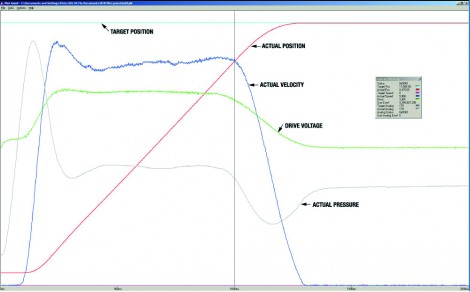
Active damping includes several methods of using feedback and a controller to electronically remove unwanted motion or oscillations. Active damping is normally required on systems that have a low natural frequency (i.e. they can be modeled like a mass on the end of a spring) and a high static to dynamic friction ratio. In these applications, the force builds up across the piston until the static friction force is overcome and the piston starts to move. When the piston moves, the force across the piston falls below the dynamic friction force and the piston stops. Figure 2 contains the motion plot of an actively damped system running an I-PD control algorithm. Any system that suffers from this stiction or chatter when running in open-loop mode will also do the same in closed-loop mode. Borderline systems also tend to exhibit the same stiction action when in closed-loop mode. The solution is to limit the acceleration, or the rate-of-change of the force on the piston.

This is problematic as calculating the instantaneous acceleration from position transducers is usually not feasible. Instead, some method of obtaining acceleration feedback is needed. The most direct way to do this is to attach an accelerometer to the carriage or actuator that is moving the load, but this can put the accelerometer in a nasty environment, which may not be practical.

Alternatively, the differential force across the piston can be used to estimate the acceleration. This requires a controller with the necessary analogue inputs to connect to the two pressure sensors and the ability to calculate the differential force on-the-fly. This technique is not as accurate as the accelerometer approach but is commonly used and very effective at solving the stiction or chattering problem described previously. Active damping reduces the rate of force buildup across the piston and works best where the objective is to get from one point to another as smoothly as possible. Of course, active damping also limits the maximum acceleration and deceleration, which in turn limits the ability to follow a motion profile. If this is the primary objective, then larger diameter cylinders should be considered in order to increase the natural frequency, which reduces the effects of any stiction.

Another method of setting up an active damping control algorithm is to use a model-based control system that can internally estimate accurate accelerations. The advantage is that no extra hardware is required. The disadvantage is that the system must be relatively linear so that an accurate model can be developed. This explains why non-linear valve spools and pneumatic systems do not model well.

For best performance, it is better to design a hydraulic motion axis to have a high natural frequency and a linear response. But when extremely large masses must be positioned, at some point the extra expense of making the system hydraulically ‘stiff’ may become too great and electronic means are required to dampen the system.

Pressure/force control

Since fluid power is so well suited for applying pressure, a mention of pressure/force control is valuable. Today, pressure/force control (P/F) and dual-loop position-pressure/force control (P-P/F) algorithms are often used. Other systems may only need closed-loop for P/F and use open-loop for position. In some pressure applications, position PIDs can be used for pressure/force control. Other applications may need special features for combining open-loop position and single-loop P/F PID.

Dual-loop P-P/F algorithms offer more flexibility than single-loop algorithms. Since a controller cannot simultaneously fully control position and pressure, two PIDs are used, a position PID and a P/F PID, referred to together as a P-P/F PID. Both PIDs must be tuned and some method (such as a pressure threshold) used to transfer between the modes, so only one PID is operating at a time.

For many applications, a pressure limit mode is the best solution (see Figure 3). In this case, both PIDs run simultaneously, and the minimum output is used. Much can be discussed about P-P/F control and future articles will cover this topic in more depth.

Summary

Machine designers need to know that one size doesn't fit all in terms of hydraulic motion control. There are many control algorithms used in hydraulic applications, and the right one to use depends on the control needs of the application (see the table in Figure 4 for a summary). Some applications can benefit from combining two or three of the control algorithms discussed, depending on what part of the machine cycle is running. Discussing your application with the motion controller manufacturer early in the design process will help ensure that the controller has the algorithms you need.

www.deltacomputersystems.com